Fake News Detection Using LSTM Neural Networks

Considering the arduous circumstances that we all are facing in today’s world, news plays a rather significant role in our lives. We rely on it heavily to know about various domains like healthcare, politics, education, sports, etc. But there is always this problem of consuming false news. A recent study suggests that people are not only believing in false news but also it’s making them less likely to accept the real information.
In this article, we will talk about fake news detection using Natural Language Processing library(NLTK), Scikit Learn and Recurrent Neural Network techniques, in particular LSTM. We will be demonstrating the step by step explanation.
This is an introductory level article focused on the various aspects of a real-time implementation of RNN. Many of the in-depth theory aspects might not be covered in this article, but we’ll try to get the gist of it.
So let’s begin…
What is RNN?
A Recurrent Neural Network(RNN) is a type of Neural Network model where the output from a previous step is fed as input to the current step. In traditional neural networks, all the inputs and outputs are independent of each other, but in cases like when it is required to predict the next word of a sentence, the previous words are required and hence there is a need to remember the previous words. Thus RNN came into existence, which solved this issue with the help of a Hidden Layer.
The most important feature of RNN is the Hidden State, which remembers some information about a sequence. RNN has a “memory” which remembers all information about what has been calculated. It uses the same parameters for each input as it performs the same task on all the inputs or hidden layers to produce the output. This reduces the complexity of parameters, unlike other neural networks.

Sounds good? Let’s talk about LSTM.
What is LSTM and why is it used over feedback RNN?
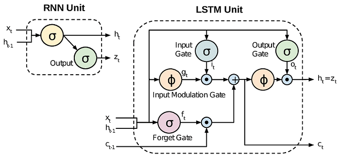
Vanilla RNNs do not have a cell state. They only have hidden states and those hidden states serve as the memory for RNNs. This lets them maintain information in ‘memory’ over time. But, it can be difficult to train standard RNNs to solve problems that require learning long-term temporal dependencies. This is because the gradient of the loss function decays exponentially with time (called the vanishing gradient problem).
LSTM networks are a type of RNN that uses special units in addition to standard units. LSTM units include a ‘memory cell’ that can maintain information in memory for long periods. A set of gates is used to control when information enters the memory when it’s output, and when it’s forgotten.

Right now. Let’s dive into our main topic of interest.
Dataset
I’m using the ‘fake news dataset’ that is available in Kaggle. The dataset can be available at this link. I imported the dataset using the read_csv function in Pandas. The dataset contains 18285 rows and 5 columns. The “label” column denotes whether the news is fake or not. 1 denotes fake news and 0 denotes true news.

In this case, we will classify the news as fake or true based on the ‘title’ column of the dataframe.
Data Cleaning and Preprocessing
The first step is to clean the dataset. The dataset contains some missing values. We drop these values using the dropna() method. Also from the dataset, we can see that the label column is our dependent feature and the rest all are independent features. So we split those independent & dependent features and store them in X and y variables respectively.
#Drop NAN values
df = df.dropna()
#Getting the independent features
X = df.drop(‘label’,axis = 1)
#Getting the dependent features
y = df[‘label’]
Let us print the shape of X and y..
print(X.shape)
print(y.shape)
The next step after cleaning up of data is the preprocessing of data. Data processing is simply the conversion of raw data to meaningful information through a process. It forms the basis for any Machine Learning/Deep Learning problem statements.
— >Importing the libraries required
import tensorflow as tf #for training of deep neural networks
from tensorflow.keras.layers import Embedding #for a real-valued vector representation
from tensorflow.keras.preprocessing.sequence import pad_sequences #to make the input length fixed
from tensorflow.keras.models import Sequential #to create a sequential model
from tensorflow.keras.preprocessing.text import one_hot #to convert sentences into one-hot representations given the vocabulary size
from tensorflow.keras.layers import LSTM #to process the sequences of data
from tensorflow.keras.layers import Dense #receives input from its previous layer
The next step is to perform stemming and removing the stopwords from the sentences.
— >Stopwords: These are the words that do not add much meaning to the sentence. We remove these stopwords from the sentences for better analysis.
Examples are : {“a”, “and”, “the”, “but”, “how,” “or”, ”what”, etc.}
— >Stemming: Process of removing the suffix from a word and reduce it to its root word. The resultant word may not be a meaningful word always.
For example:
Stemming of — > History, Historical, Historian = Histori
Stemming of — > Final, Finally, Finalized = Fina
import nltk #NLP library
import re #regular expression
from nltk.corpus import stopwords #importing stopwords
nltk.download('stopwords')messages = X.copy()   #storing the independent features
messages.reset_index(inplace = True) #since NaN values were droppedfrom nltk.stem.porter import PorterStemmer #For performing stemming
ps = PorterStemmer()
corpus = []     #list for embedding
for i in range(len(messages)):
    review = re.sub(‘[^a-zA-Z]’,' ',messages[‘title’][i])  #to create a sentence only with lower and upper case words    #lower and splitting the words
    review = review.lower().split()    #stemming all those words which are not stopwords
    review = [ps.stem(word) for word in review if not word in           stopwords.words(‘english’)]
    review = ‘ ‘.join(review)
    corpus.append(review)corpus[0:10]  #printing the first 10 sentences after stemming

So from the above output we can see that all the stop words have been removed and stemming is performed in each word of the sentences.
Now we have to convert the text data(in corpus) into one hot representations.
— >One Hot Encoding: Most of the present day ML cannot be executed on categorical data. Instead, these categorical data needs to first be converted to numerical data. One hot encoding is used to perform such operation. It is essentially the representation of categorical variables as binary vectors. These categorical values are first mapped to integer values. Each integer value is then represented as a binary vector that is all 0s (except the index of the integer which is marked as 1).
For more information, you can visit this link.
In our case, we find the one hot representation of each word with respect to the vocabulary size(vocab).
vocab=5000 #Setting up vocabulary size
onehot_repr=[one_hot(words,vocab)for words in corpus]
onehot_repr 
As we can see from the output above, the first word in sentence 1 is in the index ‘950’ of the vocabulary. Similarly the second word in sentence 1 is in the index ‘3189’ of the vocabulary.
Embedding Representation
As we might be aware of the fact that all the neural networks require to have inputs of same shape and size. However, when we pre-process these data and use the texts as inputs for our LSTM model, we can find that not all the sentences have the same length. So before actually giving these sentences to the embedding layer, we have to make these sentences of fixed length. This is where “padding” becomes necessary.
Here we are setting the sentence length as 30 and performing padding onto these one-hot representations of sentences using pad_sequences(). We are using padding as “pre”, which means it will add 0’s before the sentences, to make them of equal length.
length = 30 #Setting sentence length
embedded_docs=pad_sequences(onehot_repr,padding=’pre’,maxlen=length)
Printing the first 5 sentences..

We can see that all the sentences are of length 30 and 0’s are added at the beginning to fix their size.
Creating the LSTM Model
Before creating the model, we need to define the number of vectors/features. The model takes some input in the embedding layer and converts those into some specific number of features/vectors. So we have set that number to 40 in this case. Next we create a sequential object for the model.
In the 1st layer, an embedding layer is added. In embedding layer, the first parameter is the vocabulary size, followed by the feature size and finally the input size which is the sentence size in this case.
In the next layer, we add an LSTM layer with 100 neurons. Further since this is a classification problem, a dense layer is added with the activation function as sigmoid.
Finally we compile the model using loss function as binary cross-entropy(as only two outputs), optimizer as adam and metrics as accuracy.
#Creating the lstm model
embedding_vector_features=40
model=Sequential()
model.add(Embedding(vocab,embedding_vector_features,input_length=length))
model.add(LSTM(100)) #Adding 100 lstm neurons in the layer
model.add(Dense(1,activation=’sigmoid’))#Compiling the model
model.compile(loss=’binary_crossentropy’,optimizer=’adam’,metrics=[‘accuracy’])
Printing the model summary, we get..

Fitting the model
Here the padded embedded object X(independent features) and y(dependent features) are converted into an array and stored in variables X_final and y_final respectively.
import numpy as np
X_final=np.array(embedded_docs) # Converting X and y as array which are embedded padded objects
y_final=np.array(y)
— >Splitting the data
To test our model performance, we will perform a train_test_split into X_final and y_final variables using model_selection from sklearn package. We will split those into training data and test data with test size as 0.33.
#Train test split of the X and y final
from sklearn.model_selection import train_test_split
X_train, X_test, y_train, y_test = train_test_split(X_final, y_final, test_size=0.33, random_state=42)
Model Training
We proceed with training the model using model.fit() with parameters X_train, y_ train, the validation data as (X_test,y_test) ,the number of epochs as 10 and the batch size as 64. For each epoch, the model is evaluated on the validation_data to compute the loss.
# Fitting with 10 epochs and 64 batch size
model.fit(X_train,y_train,validation_data
(X_test,y_test),epochs=10,batch_size=64)
Here are the epochs

Model Evaluation
We predict the output(y_pred) for our test data and evaluate the predicted values with y_test. The below metrics can be used to evaluate the model:
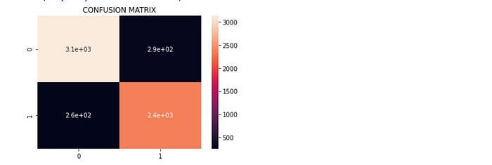
— >Confusion matrix: It is a N x N matrix used for evaluating the performance of a classification model, where N is the number of target classes. The matrix compares the actual target values with those predicted by the machine learning model.
We are using the heatmap() function from seaborn package to visualize the confusion matrix.
#Predicting from test data
y_pred=model.predict_classes(X_test) # Predicting from test data
from sklearn.metrics import confusion_matriximport seaborn as sns
import matplotlib.pyplot as plt#Creating confusion matrix
#confusion_matrix(y_test,y_pred)cm = confusion_matrix(y_test,y_pred)
ax = plt.axes()
sns.heatmap(cm,annot = True,ax = ax)
ax.set_title(‘CONFUSION MATRIX’)

— >Accuracy: It is the fraction of predictions that our model got right.
from sklearn.metrics import accuracy_score
accuracy_score(y_test,y_pred)
We are getting an accuracy of 90.85% for our model. So that indicates that our model performed fairly well.
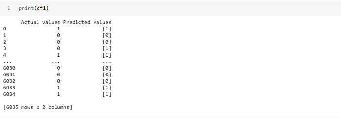
For comparison of actual values and predicted values on test data by the model, we created a dataframe. We converted the test data(arrays) to list and then to dictionary. Now dataframe is created with the dictionary.
list1=y_test.tolist() #array to list
list2=y_pred.tolist()
d={“Actual values”:list1,”Predicted values”:list2} #list to dict
df1=pd.DataFrame(d) #dictionary to dataframe
Printing the dataframe..

Summary
In this article, we have learned about a use case example of fake news detection using Recurrent Neural Networks(RNN) in particular LSTM. We implemented various steps like loading the dataset, cleaning & preprocessing data, creating the model, model training & evaluation, and finally accuracy of our model.
For more in-depth intuition about LSTM, you can refer this wonderful post: Understanding LSTM Networks
We hope you enjoyed this article!
Authors: B.Sahithi Reddy, A.Umashankar Rao, Jayanta Kumar Pal
Code Link: The whole code for this article can be found in this GitHub link.
